DESCRIBE THE STRENGTH AND DIRECTION OF THE LINEAR CORRELATION

When the points of a scatter plot are clustered along a line, we say there is a linear correlation between the quantities represented by the data.

Problem 1 :

A group of male children were weighed. Their ages and weights are recorded in table.

(i) Draw the scatter plot of these data .

(ii) Describe the strength and direction of the correlation between the age and weight.

Solution :

(i) Scatter plot of the data :

(ii) There is strong positive correlation between age and weight.

Problem 2 :

The table below shows the average number of additional years a U.S. citizen is expected to live for various ages.

(a) Draw a scatter plot of these data.

(b) Writing to Learn Describe the strength and direction of the correlation between age and life expectancy.

Solution :

(i) Scatter plot

(ii) There is no linear relationship between age and remaining life expectancy.

Describe the strength and direction of the linear correlation.

Problem 3 :

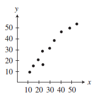
Solution :

There is strong positive linear correlation.

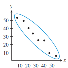
Problem 4 :

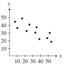
Solution :

Strong negative correlation.

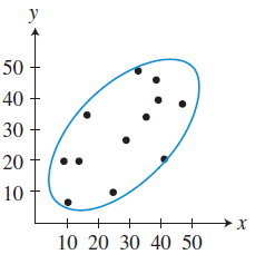
Problem 5 :

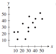
Solution :

There is weak positive linear correlation.

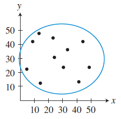
Problem 6 :

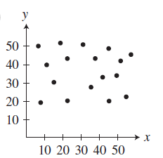
Solution :

There is no linear correlation between the quantities.

Problem 7 :

What is the correlation for the following scatter plot

a) weak positive       b)  strong negative     c) strong positive       d) No correlation

e)  weak negative

Solution :

There is no correlation. Option d is correct.

Problem 8 :

The table shows the durations x (in minutes) of several eruptions of the geyser Old Faithful and the times y (in minutes) until the next eruption.

(a) Use a graphing calculator to find an equation of the line of best fit. Then plot the data and graph the equation in the same viewing window.

(b) Identify and interpret the correlation coefficient.

(c) Interpret the slope and y-intercept of the line of best fit

Use the equation of the line of best fit.

a. Approximate the duration before a time of 77 minutes.

b. Predict the time after an eruption lasting 5.0 minutes.

Solution :

Step 1 :

Enter the data from the table into two lists.

Step 2 :

Use the linear regression feature. The values in the equation can be rounded to obtain y = 12.0x + 35.

Step 3 :

Enter the equation y = 12.0x + 35 into the calculator. Then plot the data and graph the equation in the same viewing window.

b. The correlation coeffi cient is about 0.979. This means that the relationship between the durations and the times until the next eruption has a strong positive correlation and the equation closely models the data, as shown in the graph.

c. The slope of the line is 12. This means the time until the next eruption increases by about 12 minutes for each minute the duration increases. The y-intercept is 35, but it has no meaning in this context because the duration cannot be 0 minutes.

a.

y = 12.0x + 35

77 = 12.0x + 35

77 - 35 = 12x

42 = 12x

x = 42/12

x = 3.5

An eruption lasts about 3.5 minutes before a time of 77 minutes.

b. Use a graphing calculator to graph the equation. Use the trace feature to find the value of y when x ≈ 5.0, as shown.

A time of about 95 minutes will follow an eruption of 5.0 minutes.

Problem 9 :

Tell whether a correlation is likely in the situation. If so, tell whether there is a causal relationship. Explain your reasoning.

a. time spent exercising and the number of calories burned

b. the number of banks and the population of a city

Solution :

a. There is a positive correlation and a causal relationship because the more time you spend exercising, the more calories you burn.

b. There may be a positive correlation but no causal relationship. Building more banks will not cause the population to increase.

Problem 10 :

The table shows the mileages x (in thousands of miles) and the selling prices y (in thousands of dollars) of several used automobiles of the same year and model.

a. Use a graphing calculator to find an equation of the line of best fit.

b. Identify and interpret the correlation coefficient.

c. Interpret the slope and y-intercept of the line of best fit.

d. Approximate the mileage of an automobile that costs $15,500.

e. Predict the price of an automobile with 6000 miles.

Solution :

a)

b) Correlation coefficient

R² = 0.9379

r = -0.9379

c)  y = - 0.18x + 19.71681

Slope = 0.18

y-intercept = 19.71681 (1000) ==> 19716.81

y = -0.180x + 19716.81

d.  Approximate the mileage of an automobile that costs $15,500.

15500 = - 0.18x + 19716.81

15500 - 19716.81 = -0.18x

-4216.81 = - 0.18x

x = 4216.81/0.18

x = 23426.7 miles

e. Predict the price of an automobile with 6000 miles.

y = -0.18(6000) + 19716.81

y = -1080 + 19716.81

= 18636.81